[Jodavaho.io]

OK, let’s talk about my diet some more.

I’ve started a diet, with the goal of losing 32 lbs, or ~15% of my bodyweight, to get back to my circa 2000-2005 weight. I’m happy if I achieve 80% of that loss, ending up under 200. This is a long post, in which I describe the plan, and some misunderstandings I had about dieting and weight loss.

Along the way, I built an estimator that uses data to determine my real calorie intake, needs, and activity level. In practice, the hardest part about calorie deficits is tracking calories. Burying the lede a little, it turns out LLM / ChatGPT-4 is fantastic at counting calories for you from pictures, descriptions, or rough notes.

This is part two of a series. The first part disucsses basic math for calorie needs and steady state weight, and is here.

What’s a diet

My definition of diet is extended calorie deficit for the purposes of losing bodyfat. I do not differentiate types of food, but I prefer high protein for appetite control. I also don’t do time-based restriction, though I find that skipping breakfast and not eating after dinner is sustainable, and that’s roughly an 18/6.

From the first part, we have a few equations to work with:

1. Mifflin-St Jeor¹ $ BMR = 10 \times weight(kg) + 6.25 \times height(cm) - 5 \times age(y) + G$, where $G$ is 5 for men, and -161 for women.
2. $TDEE = BMR \times L$, where $L$ is a multiplier for your daily activity level.

Hereafter, shortened to

$$ \begin{aligned} BMR =& 10 w + 6.25 H - 5A + G \\ TDEE =&L \cdot BMR\\ &\text{ with } L \in \{1.2, 1.375, 1.55, 1.725, 1.9\} \end{aligned} $$

We also know we can calculate the steady state weight, which is the weight at which you will neither gain nor lose weight. This is a function of your activity, age and height, and the calories you consume.

$$ \begin{aligned} SSW &= \frac{cal - L\cdot [6.25 H - 5 A + G]}{10} \\ \end{aligned} $$

See part 0 for more details.

From this we’re accumulating python code:

from enum import Enum

def bmr_m(weight, height, age):
    return 10 * weight + 6.25 * height - 5 * age + 5

def bmr_f(weight, height, age):
    return 10 * weight + 6.25 * height - 5 * age - 161

class Activity(Enum):
    SEDENTARY = 1.2
    LIGHT = 1.375
    MODERATE = 1.55
    VERY = 1.725
    EXTRA = 1.9

def calc_tdee(bmr, activity):
    """
    Calculate Total Daily Energy Expenditure
    """
    if (activity < 1.2 or activity > 1.9):
        raise ValueError("Activity must be between 1.2 and 1.9")
    return bmr * activity

def steady_state_weight(calories, activity, height, gender, age):
    """
    Reverse BMR to find weight given calories
    """
    L = activity
    if gender=='m':
        wt = calories /  L - (6.25 * height - 5 * age + 5)
        wt = wt / 10
        return wt
    if gender == 'f':
        wt = calories /  L - (6.25 * height - 5 * age - 161)
        wt = wt / 10
        return wt
    raise ValueError('sex: m|f only')

We left of with the big question: how long does it take for the effects to be fully realized? Now, let’s figure that out, and, that will allow me to, answer, if I want to lose 30 lbs by mid-summer, how many calories do I need to cut?

Deriving a predictive model for weight loss

Alright, using only BMR / TDEE, what can we say about weight loss over time?

Given weight loss is a function of the difference between TDEE and calories, thinking it through, if we’re far from our target weight, the difference between TDEE and our calorie intake is large, so we should shed weight quickly. As we approach our target weight, the difference shrinks, and we should lose weight more slowly.

Let’s plot this. Assuming a 300 calorie deficit will shed $300/7700$ kgs, we have:

def wt_change(calories, tdee):
    """
    Given calories consumed, and calculated TDEE (using kg!), how much weight
    will you lose?

    Returns delta-weight in kg
    """
    calories_per_kg = 7700
    return (calories - tdee) / calories_per_kg

And so:

def predict_wt(days, ht, age, wt0, calorie_target, activity=Activity.SEDENTARY.value):
    """
    Given you want to cut calories by calorie_cut below your starting BMR, over
    the range of days, what will your weight be?

    Accepts wt0 in kg, ht in cm, age in years
    Returns a list of weights over time in kg
    """
    wts = [wt0]
    for i in range(1, days):
        current_wt = wts[-1]
        bmr = calc_bmr(current_wt, ht, age, 'm')
        tdee = activity * bmr
        dwt = wt_change(tdee, calorie_target)
        wts.append(wts[-1] + dwt)
    return wts

And if we plot out the weight loss over 3 years, we get:

def plotxy(x,y):
    import plotille as plt
    fig = plt.Figure()
    fig.width = 40
    fig.height = 10
    fig.plot(x, y)
    print(fig.show())

wts = predict_wt(365*3, to_cm(77), 43, to_kg(222), 2100)
plotxy(range(0, 365*3), wts)

And the result is:

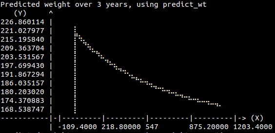
Well, it definitely flattens out. And for my taste, that’s far too slow in the second or third year. When do we reach our SSW? Well, never, actually. We asymptotically approach it. So to get something like linear progression, you want to be the early stages, where the difference between TDEE and calories is large.

Light bulb #3: If you want to hit your target weight, you have to aim past it. If you want to hit it quickly, you have to aim far past it.

That gradual flattening out is a classic exponential decay. The equation for “weight over time” must certainly be of the form $w(t) \propto w_0 e^{-kt}$, where $w_0$ is the initial weight, $k$ is the decay constant, and $t$ is time.

I can happily continue plotting by iterating over days, but that’s not very fun, and I distrust my discrete simulation skills. Let’s derive the equation. Let’s start with the “Delta Weight” equation, and see if we can integrate that to find the weight over time.

$$ \frac{dw(t)}{dt} = \frac{calories - tdee(t)}{7700} $$

Expanding that out, we get (using the $TDEE$ equation from above):

$$ \frac{dw(t)}{dt} = \frac{cal - L (10 w(t) + 6.25 H - 5 A + G) }{7700} $$

Where $cal$ is the calories, $L$ is the activity level, $w(t)$ is the weight at time $t$, $H$ is height, $A$ is age, and $G$ is the “gender constant” from the BMR equation.

The fact that we have $dx/dt$ on one side and $x$ on the other is a hint that this is a first order linear differential equation. You can use automated tools to solve this, but it will generally be ugly if you don’t prepare the equation first.

So, we can prepare and solve it by separation of variables². We can break out $w(t)$ and tuck some constants away to get:

$$ \frac{dw(t)}{dt} = \frac{C}{B} - \frac{10L}{B} w(t) $$

where $C = cal - L [6.25 H - 5 A + G] $ and $B = 7700 $. This can be separated to:

$$\begin{aligned} &\left(\frac{1}{ \frac{C}{B} - \frac{10L}{B} w(t) }\right) dw(t) = dt\\ &\left(\frac{B}{ C - 10L w(t) }\right) dw(t) = dt \end{aligned}$$

Wolfram Alpha made me dig way back to Calc II u-substitution, with $u = C - 10L w(t)$, and $du = -10L dw(t) \implies dw(t) = \frac{1}{-10L} du$. Subbing those in, we get:

$$\begin{aligned} \left(\frac{B}{ u }\right)\frac{1}{-10L} &du(t) = dt \\ \left(-\frac{B}{ 10L }\right) &\frac{du(t)}{u} = dt \end{aligned}$$

And since $\int\frac{du}{u} = ln(u) + K$¹, we have $=ln(C-10Lw(t)) + K$ so we get:

$$\begin{aligned} -\frac{B}{10L} ln(C-10L w(t)) &= t + K \\ ln(C-10L w(t)) &= -\frac{10L}{B} (t + K)\\ C-10L w(t) &= e^{-\frac{10L}{B} (t + K)}\\ w(t) &= \frac{C - e^{-\frac{10L}{B} (t + K)}}{10L}\\ w(t) &= \frac{C}{10L} - e^{-\frac{10L}{B}(t)} \left(\frac{e^{-\frac{10LK}{B}}}{10L}\right) & \text{❓ ugly…} \\ \end{aligned}$$

Note that $K$, the integration constant, is hiding up there. Let’s use initial conditions of $w(0)$ to find solve the previous equation to eliminate arbitrary constants.

$$\begin{aligned} w(0) &= \frac{C}{10L} - e^{-\frac{10L}{B}(0)} \left(\frac{e^{-\frac{10LK}{B}}}{10L}\right) \\ w(0) &= \frac{C}{10L} - \frac{e^{-\frac{10LK}{B}}}{10L} \\ 10 L w(0) &= C - e^{-\frac{10LK}{B}}&\text{ } \\ e^{-\frac{10LK}{B}} &= C - 10 L w(0)&\text{✅ } \\ %e^{-\frac{10LK}{B}} &= cal - L[6.25 H - 5 A + G ] - 10 L w(0) \\ %e^{-\frac{10LK}{B}} &= cal - L [6.25 H - 5 A + G + 10 w(0)] \\ %e^{-\frac{10LK}{B}} &= cal - TDEE(0) \\ %-\frac{10LK}{B} &= ln(cal - TDEE(0)) \\ %K &= \frac{-B}{10L} \cdot \text{ln}(cal - TDEE(0))/(10L)&\text{✅ Solved K} \\ %\implies e^{-\frac{10LK}{B}} &= cal - TDEE &\text{✅ Simplifies!} \\ \end{aligned}$$

That’s nice! So subbing back, we have just solved $w(t)$ as:

$$\begin{aligned} w(t) &= \frac{C}{10L} - e^{-\frac{10L}{B}(t)} \left(\frac{e^{-\frac{10LK}{B}}}{10L}\right) &\text{} \\ w(t) &= \frac{C}{10L} - e^{-\frac{10L}{B}(t)} \left(\frac{C-10Lw_0}{10L}\right) & \text{} \\ \end{aligned}$$

Now, $C$ is a constant I introduced, with value $cal - L[6.25 H - 5 A + G]$, and $B$ is the 7700 calories per kg. This means:

$$ \begin{aligned} \frac{C}{10L} &= \frac{cal - L[6.25 H - 5 A + G]}{10L} &\text{} \\ \frac{C}{10L} &= SSW\text{} \\ \end{aligned} $$

Let’s expand, using $SSW$ for $C/10L$:

$$ \begin{aligned} w(t) &= \frac{C}{10L} - e^{-\frac{10L}{B}(t)} \left(\frac{C-10Lw_0}{10L}\right) & \text{} \\ w(t) &= SSW - e^{-\frac{10L}{B}(t)} \left(SSW -w_0\right) &\text{} \\ \\ w(t) &= SSW\cdot\left(1-e^{-\frac{10L}{B}(t)} \right)+ w_0 e^{-\frac{10L}{B}(t)} &\text{[✅] closed form!} \\ w(t) &= SSW + (w_0 - SSW) e^{-\frac{10L}{B}(t)} &\text{[✅] smaller form!} \\ &\text{w/ }SSW=cal - L[6.25 H - 5 A + G]/10L &\text{} \\ \end{aligned} $$

OK, so we have a closed form equation for weight over time. With time = 0: $$ \begin{aligned} w(0) &= SSW + (w_0 - SSW) e^{-\frac{10L}{B}(0)} &\text{} \\ w(0) &= SSW + (w_0 - SSW)\cdot 1 &\text{} \\ w(0) &= w_0 &\text{} \\ \end{aligned} $$

… it gives us our starting weight, and as time goes to infinity:

$$ \begin{aligned} w(\infty) &= SSW + (w_0 - SSW) e^{-\frac{10L}{B}(\infty)} &\text{} \\ w(\infty) &= SSW + (w_0 - SSW) \cdot 0 &\text{} \\ w(\infty) &= SSW &\text{} \\ \end{aligned} $$

… it gives us our steady state weight. Perfect!

import numpy as np

def weight_over_time(days, calories, 
                     ht, age, wt0, 
                     activity=Activity.SEDENTARY.value):
    """
    Given you want to consume `calories` per day, over the range of days, what
    will your weight be?

    Accepts wt0 in kg, ht in cm, age in years
    Returns a list of weights over time, one per day, in kg
    """
    SSW = steady_state_weight(calories, activity, ht, 'm', age)
    t = np.arange(0, days)
    exparr = np.exp(-10*activity/7700* t)
    res = SSW + exparr * (wt0-SSW)
    return res

OK, let’s have a look! Given my weight loss goal, target calories, and starting weight, we can plot it out!

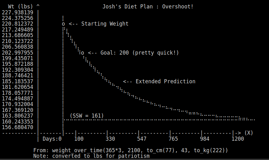
My current calorie goal / activity level goal combine to give a $SSW$ of 161 lbs. This is the weight I would asymptotically approach if I ate 2100 calories per day and maintained my current activity level, and represents a weight loss of 61 lbs.

Give my goal was to lose 32 lbs, I massively overshot my goal weight with this calorie / activity level. This is intentional, to lose weight quickly. After reaching ~190 or so, I’ll probably switch to a sustainable level of food/activity (if I even can). But who knows? Now I know.

This is probably not super healthy. I suspect this is what most people have in mind when they think “diet” - something that moves quick by massive over-compensation.

Light bulb #4: A more sustainable diet is to pick calories given steady-state-weight and activity level, and let years do the work

Note, given all the closed form equations above, it’s natural to start plugging in different parameters and solving for different things. Let’s do that next.